Introduction
The goal of this project was to use a combination of the 50-day and 20-day simple moving average (SMA) and a deep learning algorithm to predict the adjusted close price for the next day of a stock based on data from the current day of that stock.
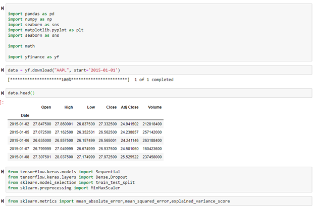
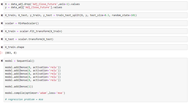
To begin, all the standard libraries being used for the stock projects were imported as well as the Tensorflow and sklearn models shown below.
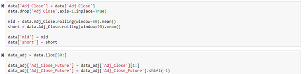
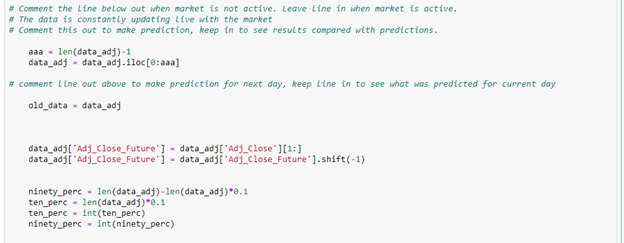
Next, the 50-day SMA and 20-day SMA were calculated and added onto the data frame. The data frame was then sliced to take out all of the NaN values in the 50-day and 20-day SMA columns. Since the purpose of this project was to predict the adjusted close price of the next day based on data from the previous day, the “Adj_Close_Future” column was added to place the adjusted close price from the next day onto the current day.
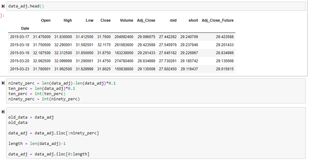
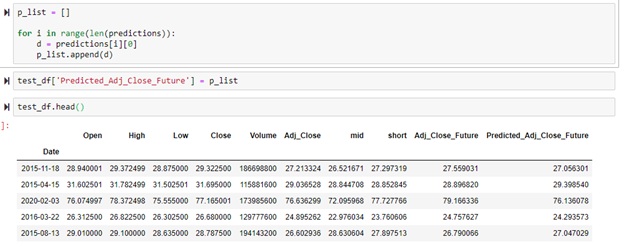
Below shows the top of the new data frame. The data was split into the first 90% and into the last 10%. The model was trained and internally tested on the first 90%. Once the model had been created for the first 90%, the model was used to determine accuracy on the last 10% of the data to see how the model would perform on a completely new dataset range.
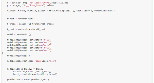
The deep learning model was created below. The data was appropriately scaled using MinMaxScaler. The rectified linear unit (relu) activation function combined with the adam optimizer and 6 layers that have 8 nodes each was the best combination that was determined through trial and error.
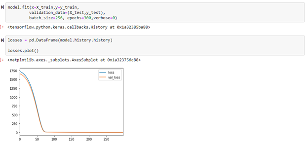
The loss and validation loss were both plotted below to determine if the model was overfitting or underfitting. The graph shows the plot of training loss and validation loss both decreasing to the point of stability which means that the model is a good fit.
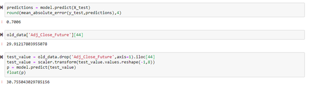
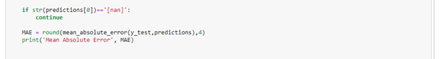
After the model had been created and the graph of losses showed a good fit, the mean absolute error was calculated to get an idea of the accuracy. The mean absolute error was calculated to be 0.7. This means that on average, the model predicted the adjusted closing price within $0.7 of the actual adjusted close price. Given that the adjusted close price is consistently above $30 in the dataset, this is a very good result. Based on a $30 adjusted close price, the model guessed the value within 2.3% (0.7/30 = 0.023). The code below also shows a comparison between an actual value of $29.9 and a predicted value of $30.7 which is extremely close.
The purpose of this project is to predict an increase or decrease in value for the next day of the stock. The model was used to predict what the adjusted close will be, and those predictions can be used to determine whether the stock went up or down the next day. The X_test data frame contains the data that the model has not seen yet so this is the data that will be tested. I transformed the X_test data frame into the test_df data frame by creating a list of all the opening costs in the X_test data frame and using that list to find all of the dates in the data_adj data frame that matched those opening costs. The predictions were then calculated using model.predict from the model that was previously created.
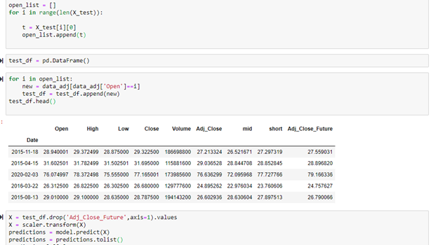
The predictions output an array with two embedded lists. The predictions were then sent to a list and the second embedded list was removed using the for loop below. Once the correctly formatted predictions list was created, it was added onto the test data frame.
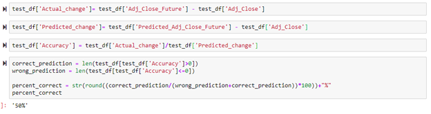
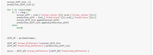
To determine whether the stocks value went up, the adjusted close price was subtracted from the future adjusted close price. This was done for predicted future adjusted close price and actual future adjusted close price. If the price went up, a positive value occurs. If the price went down, a negative value occurs. The actual change and predicted change columns were then divided by each other to create the accuracy column. If a value in the accuracy column is positive, the adjusted close price was predicted correctly. If a value in the accuracy column is negative, the adjusted close price was predicted incorrectly. This is the case because if the actual change and the predicted change share the same sign (positive or negative), then dividing by each other will create a positive number indicating that the prediction was correct. To determine the overall accuracy, the number of times the prediction was correct was divided by the total amount of times a prediction occurred. This resulted in an accuracy rate of 50%. This accuracy was mediocre so this model was used to make predictions on the 10% of the data set that was sliced out originally to see if there would be any difference.
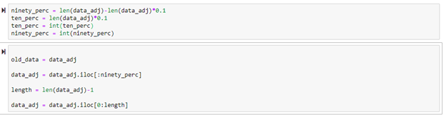
As mentioned and shown earlier, the data was broken into 90% and 10% to see how the model would perform on completely new data.
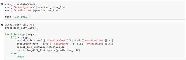
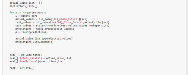
A list of the actual future adjusted close prices was created, and a list of the predicted adjusted close prices was created.
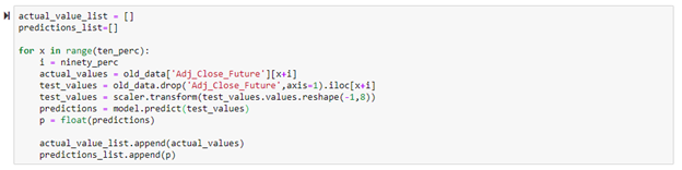
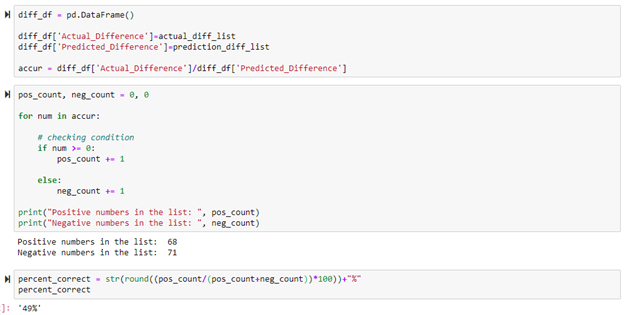
A data frame was then created, and these lists of values were added to it. The difference from day to day in future adjusted close price for actual and predicted were made into a list.
The same method previously used to determine the number of times the model predicted correctly was used here. On this new set of data from the Apple stock data set, the model again predicted about 50% correctly.
New Theory Based on Results
After these conclusions were made, I developed a theory that this model could work differently for different stocks. For example, this model could be more accurate for certain stocks and less accurate for other stocks. To test this theory, I decide to run this model over a list of stock tickers to see what the performance for each stock would look like.
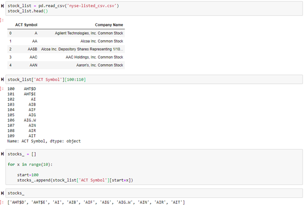
To begin, I found the CSV file online that includes a list of all the stocks on the New York Stock Exchange and their respective ticker symbol. I sliced the data to create a list of 10 stocks to test. This program can be ran over hundreds of stocks, but the more stocks included, the longer the program takes to output the results.
To see the full code of the cell I am about to break down please click link below.
This code is extremely similar to the code that was previously shown. The main difference is that this code was included in one large cell so that the code could be ran over multiple stocks at once by just running the cell one time. To begin, I initialized all the lists I would eventually create a data frame out of. The 50-day and 20-day SMA were calculated to start. Some of the stocks in the CVS file I downloaded were not on the New York Stock Exchange anymore. To keep the program running and not stopping from an error, I included the two if statements below which tell the program to keep running if no data is found for that respective stock.
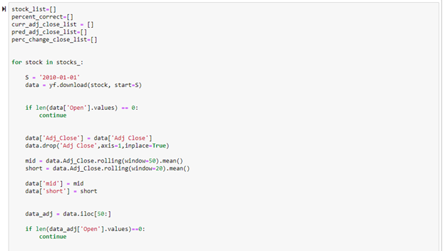
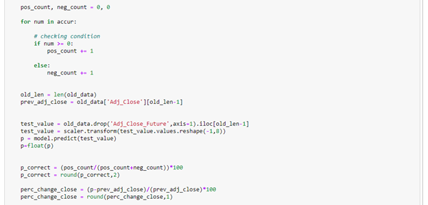
This portion of the code below is extremely crucial to testing the effectiveness of this examination. When the two lines between the comments are commented out, the program makes a prediction for the next day that has not occurred yet. When the two lines between the comments are not commented out, it makes a prediction for the current day or it makes a prediction for an adjusted close price that has already occurred. This is setup this way to compare the prediction to the actual value of the most current day to see truly if the program made the right prediction. This code portion also shows the creation of the 90% length and the 10% length.
The code below shows the deep learning model being created.
For some of the predictions made on stocks that do not have complete data sets in Yahoo Finance when imported from the CSV, NaN values would occur and this would cause the code to stop due to an error. To combat this, the if statement below was created to let the program continue. The first test of accuracy was also created here by mean absolute error.
The code below is virtually the same code that was previously shown, but these were include all in one cell to make predictions on a list of stocks. This section was used to compare the accuracy of the predictions with the actual values.
This portion below shows the accuracy by checking if the stock went up or down. Also, the predicted percent change was calculated here based on the model’s prediction of the adjusted close price.
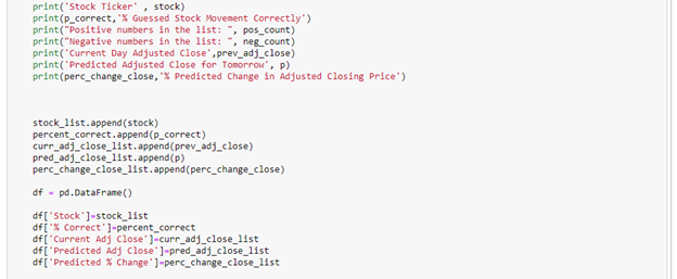
Below shows the last lines of code in the cell. The printing was included to see the output of the code in real time as it iterated through each of the stocks. The data frames were created to easily access all of the data from one area to perform further analysis and comparisons.
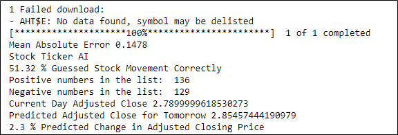
Here is a portion of the output of the code as it is running. As you can see, there was a failed download due to the stock being delisted. Since the if statements were included to make the program continue running, no error occurred. After the failed download, stock ticker AI was successfully imported, and the analysis was ran on it.
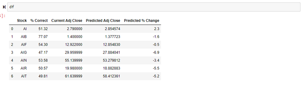
The final data frame created is shown below. As you can see, the percent predicted correctly varies from stock to stock with some stocks predicting the values correctly more than others.
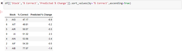
Since only 10 stocks were analyzed this go around, it is easy to see which stock predictions performed better. For a longer list of stocks, organizing the data helps to better see which stock predictions performed the best. Sorting the values on % Correct is a great way to determine which is the most accurate.
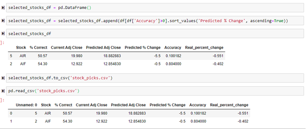
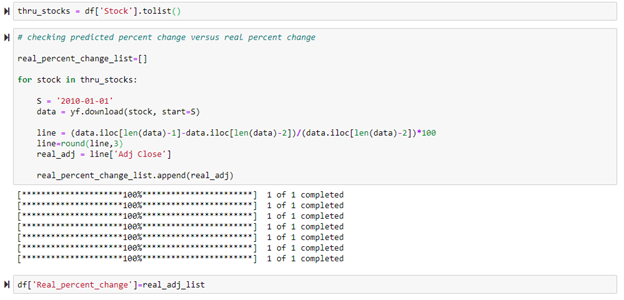
The goal is to accurately predict if the stock is going to go up or down for the next day based on predicted the adjusted close price. The stocks that successfully made it through the model and had predictions made were added to the thru_stocks list shown below. Since the Yahoo Finance API does not show the percent change, the for loop below was used to calculate the actual percent change for each of the stocks.
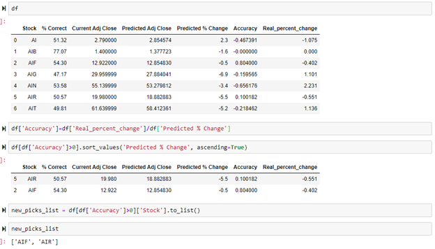
After the real percent change was calculated, it was compared with the precited percent change to determine the accuracy. Once the accuracy column was calculated, a new list was created for all stocks that the price movement was correctly predicted. As shown below, the stock tickers AIR and AIF correctly predicted the movement of the stock for the next day. AIF, overall, had the best results. This stocks movement was predicted correctly 54% of the time, the model predicted the most recent movement of the stock correctly, and the predicted percent change and real percent change for the most recent day were extremely close to each other. Based on the results of this model, AIF would be the best stock to further analyze to determine if it is currently a good investment. AIR guessed the stock movement correctly for the most recent day, but with an overall percent correct of just 50% it is more risky.
If this program were run over hundreds of stocks, more than just these two stocks would have correctly predicted the stock movement for the most recent date. When that is the case, the stocks that performed the best need to be saved and then imported the next day to repeat this whole process. This can be done by exporting a data frame of the best performing stocks to CSV files so they will be saved and ready to be imported the following day. Below shows the process of exporting and importing the best performing stocks.