Introduction

The explanation of this project in this webpage is meant to be a technical explanation of the underlying code and ideas behind the project. If you are interested in seeing the big picture version, please go to the video presentation that can be found here Video Presentations.

The purpose of this project was to create a Startup company that uses machine learning and data analysis on data from construction field reports to accurately predict the most effective means and methods to increase productivity while minimizing cost. A presentation to pitch the idea was created to generate investments from investors, as well as, procure realistic data from construction companies that are interested in proving this theoretical idea works. To see this presentation, please click here Video Presentations.

Technology Utilized

This project was constructed using the Jupyter Notebook, and Python was the base programming language used.

The main Python libraries involved in this projects creation are shown in this list.

• Pandas
• NumPy
• Matplotlib
• Seaborn
• Sklearn
• TensorFlow
• Keras

---

Dataset Invloved

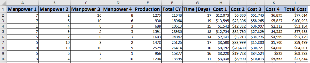
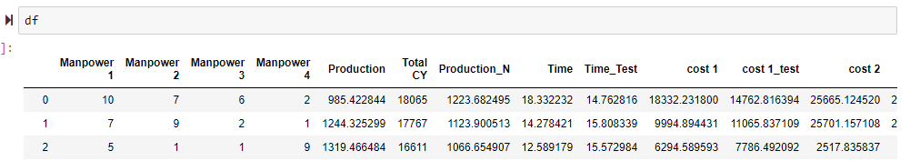
Before approaching companies for their proprietary data, the project needed to have a proof of concept. To obtain this proof of concept, a randomized data set was created. The head of the data set is shown in this table. Each row of data represents a completely unique similar construction project with varying manpower, production, materials, costs etc. Each cell under manpower 1 through 4 columns generated a random number between 1 and 10 people (this was done in excel using the formula RANDBETWEEN(1,10) ). Since production depends on manpower, the production was calculated using the sum of randomized percentages of each of the man power cells (this was done using the excel formula 100*(A2*RAND()+B2*RAND()+C2*RAND()+D2*RAND()) ). To generate a randomized amount of work that needed to be complete (Total CY or cubic yards), a total cubic yardage was calculated by selecting a random amount between the production multiplied by ten and multiplied by 20 (this was done using the excel formula RANDBETWEEN(E2*10,E2*20) ). After this randomized data had been created, the time to complete the work was found by dividing the total cubic yardage by the production (F2/E2). The cost columns are directly related to the man power columns. For example, cost 1 is the total cost for the duration of the project for manpower 1. Each of the 4 manpower columns were arbitrarily assigned costs per day. See the list for costs per day per 1 man power amount. Cost 1, 2, 3, and 4 were all calculated by multiplying man power amount by cost per day by total time. For example cost 1 in row 2 was calculated in excel by 100*A2*G2. Once each of the individual costs were calculated, they were summed to get the total cost column.

• One Manpower 1 = $100/day
• One Manpower 2 = $200/day
• One Manpower 3 = $300/day
• One Manpower 4 = $50/day

Project Functionality

Before getting into the project specifics, let’s outline what this application would look like fully developed and in use. This fully developed app would have two portion included related to databases. The first database portion would have a fully developed user interface that is connected to a SQL database (or similar database system) that allows project managers / field superintendents to directly enter the appropriate field reporting information such as man power, equipment, and production. The second database portion would be to develop an interface system that allows companies to connect to their current database that already has all of their field reporting information. Once the appropriate data pipelines are established and/or connected, the analysis can then take place.

Beginning the Analysis

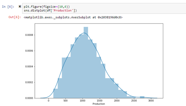
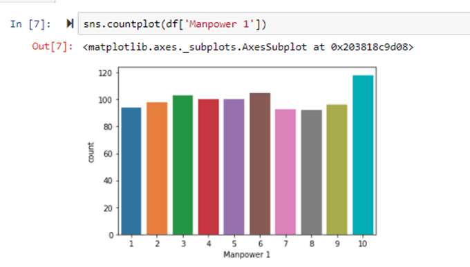
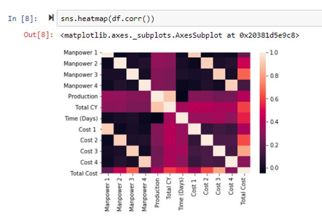
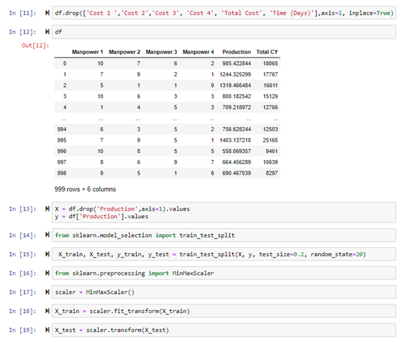
The proof of concept project began by using Pandas to import the excel dataset shown earlier. To see key relationships and acquire the best initial insights of the data, some data visualization techniques were first used.

To prepare for the creation of the machine learning model, all of the columns were dropped off the dataset besides man power, production, and total CY. The columns manpower 1, 2, 3, 4, and total CY will be used to predict the overall production. When the data was cleaned and prepared, the data was split into training and testing data to train and create the model and then test the model.

Results

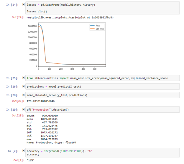
At the bottom of the previous image of code shows the model roughly had an accuracy of 16%. These results were not outstanding, but they could have been worse. Since this was a proof of concept, I am happy with the results of this project. Keep in mind that the data used in this model was completely randomized and that made extremely hard for the model to make exact predictions. In a real dataset, I believe the model would definitely pick up on reoccurring trends that would make the results much more accurate.

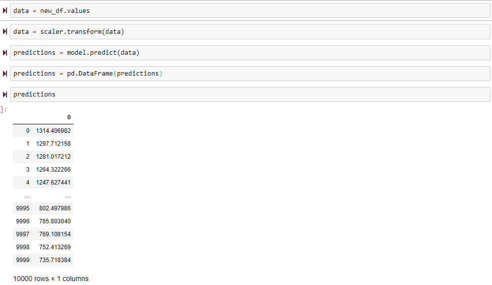
To further examine these results, the model was used to create predictions for all of the projects in the dataset.

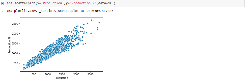
Once the predictions for all the production rates were added to the dataset, the predicted production rates were compared to the actual production rates using a scatterplot.

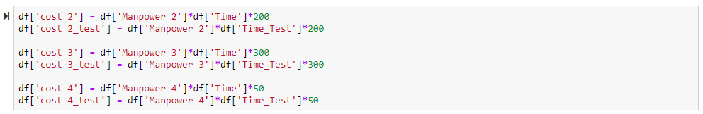
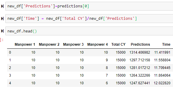
Using the predicted production rates, the predicted time and costs were found.

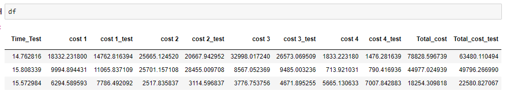
After all the predictions were added to the main data frame, further analysis was done by comparing all the predictions to the actual values.

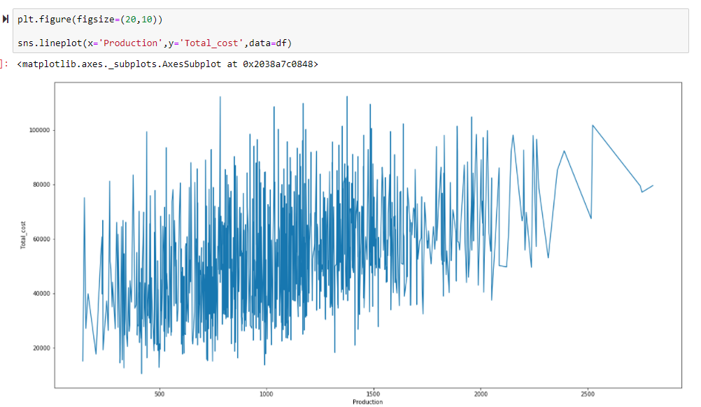
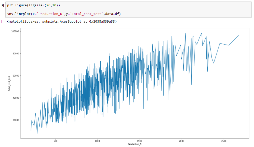
These two graphs have a lot of going on. They are showing actual production rate vs actual time and predicted production rate vs predicted time. Both of these charts show that the total cost varies significantly for a given production rate. This information is crucial for determining the optimal crew size to give the best production rate for the lowest cost.

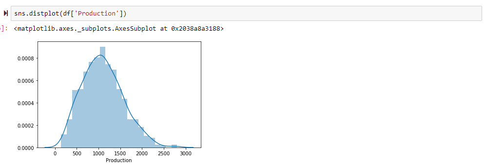
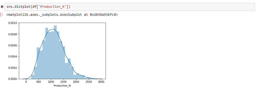
These distribution plots show that the reoccurring production rates, predicted and actual, reoccurred generally the same amount.

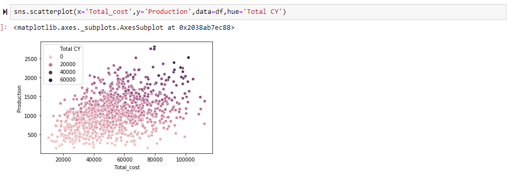
This scatterplot shows an analysis of the actual values. This chart again articulates that for a given production, there is a combination of manpower that creates a significantly lower total cost.

Conclusion

The purpose of this project was to use a machine learning model to determine the best combination of man power and equipment for a given construction project to increase production while minimizing costs for varying timeframes.

While the generated randomized data set for this project had multiple different combinations of manpower to examine, the data set did not include every possible combination of manpower. To determine the absolute best combination of manpower for a given construction project (in this example, a construction project with a certain amount of cubic yards of material to move), the model needs to be ran over every single possible combination of manpower along with the cubic yardage of material to be moved.

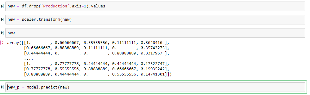
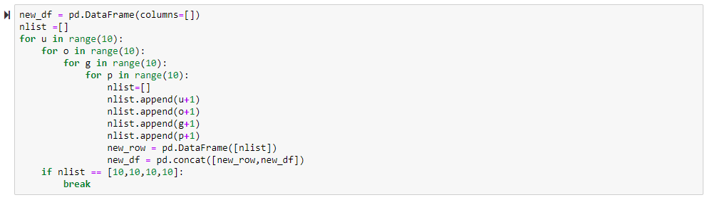
This project consisted of four different manpower options (manpower 1, 2, 3, and 4). Each of these varied in amounts of people from 1 person up to 10 people. To begin in this step of the analysis, data for all combinations of manpower needed to be created. This code shows the process for creating all possible manpower combinations.

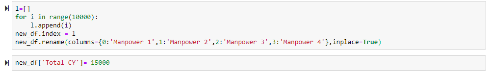
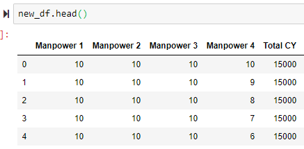
After the list was created, it was added on to a data frame. For this example, the project has a total of 15000CY that needs to be moved.

The data set created was then ran through the model that was previously created to predict production values for all of the various combinations of manpower.

The predictions of production were then used to calculate the time frame it would take to complete the project by dividing the total CY by the production.

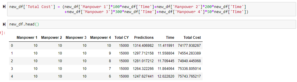
Total cost was then calculated and also added to the data frame to see how the price compared for each example project. As you would imagine, the lowest cost to complete this work would be to use 1 worker for each of the manpower columns (4 workers total). This would be the lowest cost, but would also take the longest time. Realistically, a specified duration needs to be decided on, and after that, the most cost effective combination of manpower to complete the project in that duration can be found.

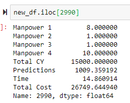
I decided to look at each of the combinations that have a duration of 15 days or less and sorted it by total cost to see which is the most cost effective.

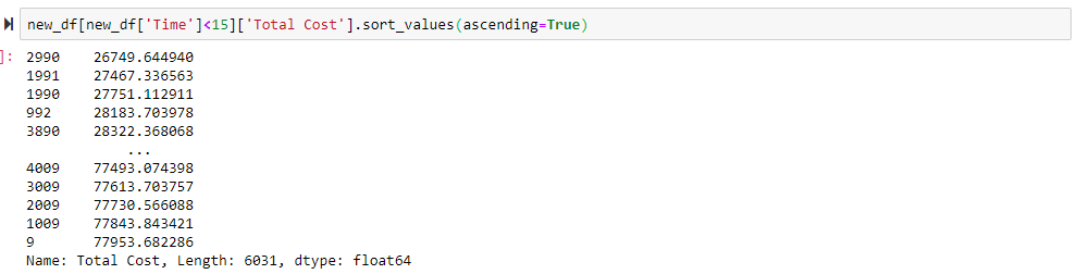
As you can see, the combination of manpower shown here gives you the cheapest option to complete the project in 15 days or less.

Thank you for taking the time to read through this project. Please check out the video presentation here Video Presentations.